Extraction example

Tutorial.

import matplotlib.pyplot as plt
import numpy as np

import tdsxtract as tx

Define sample thickness

sample_thickness = 500e-6

First we load the reference and sample signals

pos_ref, v_ref = tx.load(f"data/reference.txt")
pos_samp, v_samp = tx.load(f"data/sample.txt")
assert np.all(pos_ref == pos_samp)
position = pos_ref * 1e-6

We convert the position to time delay and plot the data

time = tx.pos2time(position)
time_ps = time * 1e12
plt.figure()
plt.plot(time_ps, v_ref, label="reference", c="#5aa2a2")
plt.plot(time_ps, v_samp, label="sample", c="#b5514c")
plt.xlabel("time (ps)")
plt.ylabel("transmitted signal (mV)")
plt.xlim(time_ps[0], 30)
plt.legend()
plt.tight_layout()

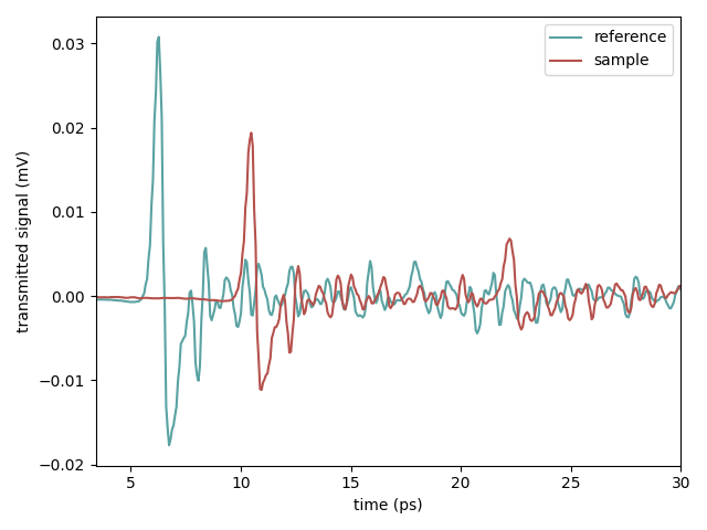
By looking at the first peak shift, we can get a rough estimate of the permittivity

eps_guess = tx.get_epsilon_estimate(v_ref, v_samp, time, sample_thickness)
print(eps_guess)

12.3904

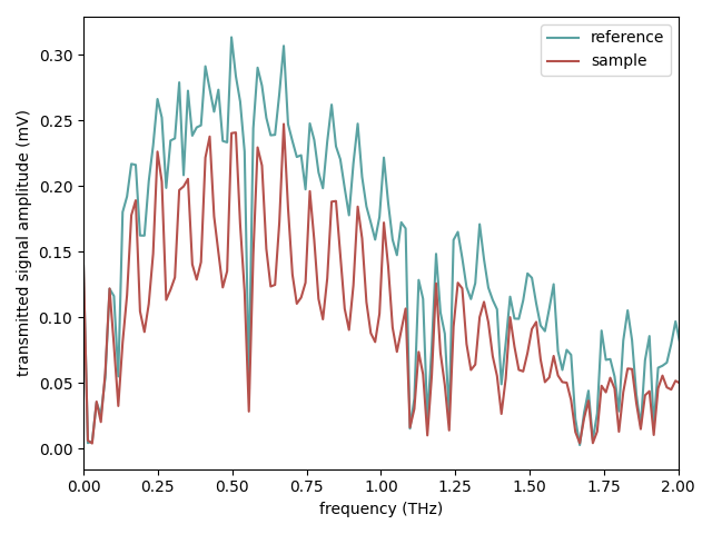
We now switch to the frequency domain by computing the Fourier transform

freqs_ref, fft_ref = tx.fft(time, v_ref)
freqs_samp, fft_samp = tx.fft(time, v_samp)
freqs_THz = freqs_ref * 1e-12


plt.figure()
plt.plot(freqs_THz, np.abs(fft_ref), label="reference", c="#5aa2a2")
plt.plot(freqs_THz, np.abs(fft_samp), label="sample", c="#b5514c")
plt.xlabel("frequency (THz)")
plt.ylabel("transmitted signal amplitude (mV)")
plt.xlim(0, 2)
plt.legend()
plt.tight_layout()

plt.figure()
plt.plot(
    freqs_THz,
    np.unwrap(np.angle(fft_ref)) * 180 / tx.pi,
    label="reference",
    c="#5aa2a2",
)
plt.plot(
    freqs_THz,
    np.unwrap(np.angle(fft_samp)) * 180 / tx.pi,
    label="sample",
    c="#b5514c",
)
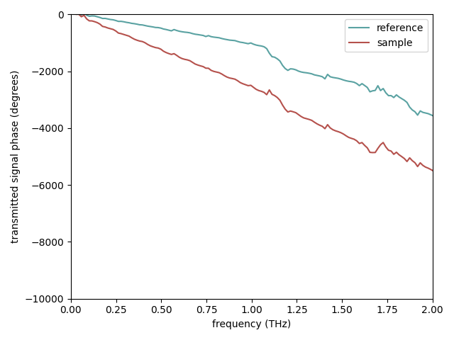
plt.xlabel("frequency (THz)")
plt.ylabel("transmitted signal phase (degrees)")
plt.xlim(0, 2)
plt.ylim(-10000, 0)
plt.legend()
plt.tight_layout()

• 
• 

Let’s calculate the transmission coefficient

transmission = fft_samp / fft_ref


#### TODO: wavelet transform check


# import pywt
# alpha = 0.01
#
# cA, cD = pywt.dwt(fft_ref, "coif4", "smooth")
# cD = pywt.threshold(cD, alpha, "soft")
# fft_ref_wl = pywt.idwt(cA, cD, "coif4", "smooth")
#
# cA, cD = pywt.dwt(fft_samp, "coif4", "smooth")
# cD = pywt.threshold(cD, alpha, "soft")
# fft_samp_wl = pywt.idwt(cA, cD, "coif4", "smooth")
# transmission_wl = fft_samp_wl / fft_ref_wl
#
#
# cA, cD = pywt.dwt(transmission, "coif4", "smooth")
# cD = pywt.threshold(cD, alpha, "soft")
# transmission_wl = pywt.idwt(cA, cD, "coif4", "smooth")
#
# transmission_wl = transmission_wl[:513]
# transmission = transmission_wl

#
# # freqs_THz, imin, imax = restrict(freqs_THz, 0.1, 2.5)
# # transmission = transmission[imin:imax]
# plt.close("all")
# plt.figure()
# plt.plot(freqs_THz, np.abs(transmission),"-")
# plt.plot(freqs_THz, np.abs(transmission_wl),"--")
# plt.xlabel("frequency (THz)")
# plt.ylabel("transmission amplitude")
# plt.xlim(0, 2)
# plt.ylim(0, 1)
# plt.tight_layout()
#
# plt.figure()
# plt.plot(freqs_THz, (np.angle(transmission)) * 180 / np.pi,"-")
# plt.plot(freqs_THz, (np.angle(transmission_wl)) * 180 / np.pi,"--")
# plt.xlabel("frequency (THz)")
# plt.ylabel("transmission phase (degree)")
# plt.xlim(0, 2)
# plt.tight_layout()


#### adapted phase unwrapping scheme: discards the noisy phase at low frequencies,
# and carries out a normal unwrapping with the reliable phase part. A missing phase
# profile at low frequencies down to DC is then extrapolated from the unwrapped phase
# at higher frequencies. In most cases the assumption of a linear phase is sufficient
# (Duvillaret et al. 1996). The whole phase profile is then forced to start at zero.
#
# phi = np.angle(transmission)
# phi_unwrapped = np.unwrap(phi)
# freqs1, imin, imax = restrict(freqs_THz, 0.1, 1)
# phi1 = phi[imin:imax]
#
# phi1_unwrapped = np.unwrap(phi1)
# fit = np.polyfit(freqs1, phi1_unwrapped, 1)
#
#
# plt.close("all")
# plt.figure()
# plt.plot(freqs_THz, phi_unwrapped)
# plt.plot(freqs1, phi1_unwrapped, "o")
# plt.plot(freqs_THz, fit[0] * freqs_THz)
# plt.plot(freqs_THz, fit[0] * freqs_THz + fit[1], "--")
# plt.show()
#
#
# plt.xlabel("frequency (THz)")
# plt.ylabel("transmission phase (rad)")
# plt.tight_layout()
#
# phi = fit[0] * freqs_THz
# transmission = np.abs(transmission) * np.exp(1j * phi)

freqs_THz, imin, imax = tx.restrict(freqs_THz, 0.2, 1.5)
transmission = transmission[imin:imax]

To describe our sample we use a Sample object

sample = tx.Sample(
    {
        "unknown": {"epsilon": None, "mu": 1.0, "thickness": sample_thickness},
    }
)

We ar now ready to perform the extraction

wavelengths = tx.c / freqs_THz * 1e-12

epsilon_opt, h_opt, opt = tx.extract(
    sample,
    wavelengths,
    transmission,
    eps_re_min=1,
    eps_re_max=100,
    eps_im_min=-10,
    eps_im_max=10,
    epsilon_initial_guess=eps_guess,
)

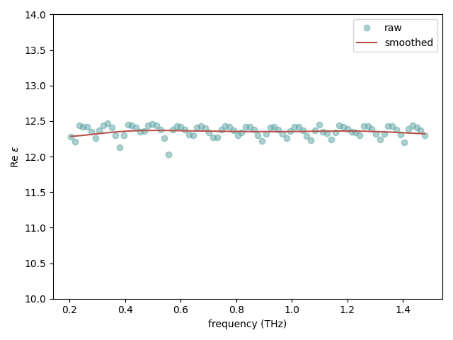
Smooth the permittivity data

eps_smooth = tx.smooth(epsilon_opt)

Plot extracted values

plt.figure()
plt.plot(freqs_THz, epsilon_opt.real, "o", label="raw", alpha=0.5, c="#5aa2a2")
plt.plot(freqs_THz, eps_smooth.real, label="smoothed", c="#b5514c")
plt.xlabel("frequency (THz)")
plt.ylabel(r"Re $\varepsilon$")
plt.ylim(10, 14)
plt.legend()
plt.tight_layout()


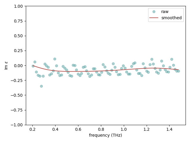
plt.figure()
plt.plot(freqs_THz, epsilon_opt.imag, "o", label="raw", alpha=0.5, c="#5aa2a2")
plt.plot(freqs_THz, eps_smooth.imag, label="smoothed", c="#b5514c")
plt.xlabel("frequency (THz)")
plt.ylabel(r"Im $\varepsilon$")

plt.ylim(-1, 1)
plt.legend()
plt.tight_layout()

• 
• 

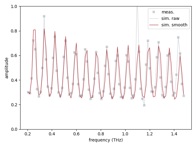
Check the transmission

t_model = tx.sample_transmission(
    epsilon_opt, h_opt, sample=sample, wavelengths=wavelengths
)

t_model_smooth = tx.sample_transmission(
    eps_smooth, h_opt, sample=sample, wavelengths=wavelengths
)


gamma = 2 * tx.pi / wavelengths
thickness_tot = sum([k["thickness"] for lay, k in sample.items()])
phasor = np.exp(-1j * gamma * thickness_tot)

fig, ax = plt.subplots()
ax.plot(
    freqs_THz,
    np.abs(transmission) ** 2,
    "s",
    label="meas.",
    alpha=0.3,
    lw=0,
    c="#656e7e",
    mew=0,
)
ax.plot(
    freqs_THz,
    np.abs(t_model) ** 2,
    "-",
    label="sim. raw",
    alpha=0.3,
    lw=1,
    c="#656e7e",
    mew=0,
)
ax.plot(
    freqs_THz,
    np.abs(t_model_smooth) ** 2,
    "-",
    label="sim. smooth",
    alpha=1,
    lw=1,
    c="#AE383E",
)

ax.set_ylim(0, 1)
ax.set_xlabel("frequency (THz)")
ax.legend()
ax.set_ylabel(r"amplitude")
plt.tight_layout()

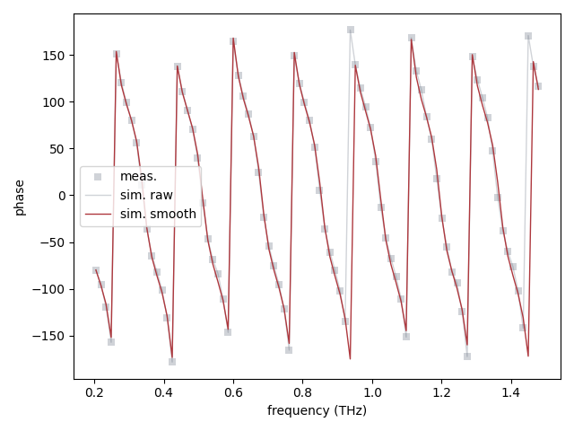
fig, ax = plt.subplots()
ax.plot(
    freqs_THz,
    (np.angle(phasor * transmission)) * 180 / tx.pi,
    "s",
    label="meas.",
    alpha=0.3,
    lw=0,
    c="#656e7e",
    mew=0,
)
ax.plot(
    freqs_THz,
    (np.angle(t_model)) * 180 / tx.pi,
    "-",
    label="sim. raw",
    alpha=0.3,
    lw=1,
    c="#656e7e",
    mew=0,
)
ax.plot(
    freqs_THz,
    (np.angle(t_model_smooth)) * 180 / tx.pi,
    "-",
    label="sim. smooth",
    alpha=1,
    lw=1,
    c="#AE383E",
)
ax.set_xlabel("frequency (THz)")
ax.legend()
ax.set_ylabel(r"phase")
plt.tight_layout()

• 
•